Are my dice random?
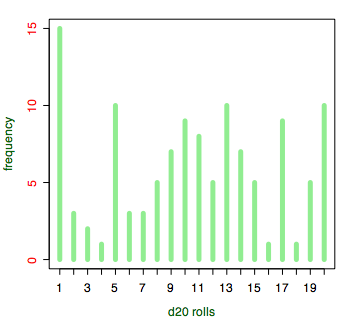
Looks fair to me. Does it look fair to you?
Gamers are a cowardly and superstitious lot. If any superhero decided to strike fear into our hearts, they would probably take on the mantle of an unlucky die. I’ve known gamers who will smash dice after bad rolls and even bury them.
The problem with eyeballing to determine whether a die is biased is two-fold. First, true randomness doesn’t look random. As humans we like to see patterns, and true randomness will look like it has patterns. Second, we tend to remember outstanding events more than others. We don’t remember the boring rolls, just the rolls that anger or delight us.
In our recent games, I’ve been playing rather than guiding, and because I’m a typically superstitious gamer, I have a special set of dice for playing. It’s a nice looking set of honey-colored dice, and I’ve never used that set until now. The d20 in that set appeared to be rolling a lot of ones. We all noticed it. After we noticed that, I started keeping track. Having seen lots of ones, I didn’t want to have to get rid of this die!
I started keeping track of the numbers after we decided it might be biased. Part of the point of running the statistics is that outstanding numbers tend to be remembered where bland numbers are not, so starting on an outstanding number is itself a bias. Here are the numbers that the suspect d20 generated over the last five gaming nights:
- 7, 18, 9, 5, 17, 20, 20, 15, 10, 9, 1, 10, 13, 5, 1, 10, 8, 5, 3, 20, 11, 14, 19, 5, 9, 13, 14, 10, 1, 15, 19, 20, 10, 14
- 9, 13, 8, 13, 7, 17, 13, 17, 11, 17, 14, 2, 14
- 6, 1, 1, 14, 19, 20, 1, 13, 20, 1, 16, 1, 15, 5
- 12, 9, 17, 10, 11, 13, 17, 9, 3, 1, 2, 14, 8, 17, 12, 2, 11, 13, 17, 10, 4, 6, 19, 5, 11, 6, 1, 5
- 12, 10, 7, 19, 1, 13, 10, 5, 1, 11, 9, 20, 17, 15, 15, 12, 8, 1, 13, 1, 5, 8, 20, 1, 11, 5, 11, 20, 20, 12
Eyeballing it, I’m seeing several ones and twenties in there. It looks pretty random to me. I’d guess that the average is right about where it’s supposed to be. But how can I tell for sure that this die is or is not biased?
The common way of testing dice for bias (besides counting up the numbers or, worse, relying on a memory of outstanding events) is the chi-square test. There is some free statistical software from the R Project for statistical computing that will help us perform this test without having to do all of the math ourselves. R is basically a scripting language specifically for statistics. It is hellaciously complicated, but for our purposes we can get by with a few lines.
What I need first is the frequency of each result. That is, 1 appeared fifteen times, 2 appeared three times, 3 appeared twice, etc. Download R and paste in the following lines:
- session1 = c(7, 18, 9, 5, 17, 20, 20, 15, 10, 9, 1, 10, 13, 5, 1, 10, 8, 5, 3, 20, 11, 14, 19, 5, 9, 13, 14, 10, 1, 15, 19, 20, 10, 14)
- session2 = c(9, 13, 8, 13, 7, 17, 13, 17, 11, 17, 14, 2, 14)
- session3 = c(6, 1, 1, 14, 19, 20, 1, 13, 20, 1, 16, 1, 15, 5)
- session4 = c(12, 9, 17, 10, 11, 13, 17, 9, 3, 1, 2, 14, 8, 17, 12, 2, 11, 13, 17, 10, 4, 6, 19, 5, 11, 6, 1, 5)
- session5 = c(12, 10, 7, 19, 1, 13, 10, 5, 1, 11, 9, 20, 17, 15, 15, 12, 8, 1, 13, 1, 5, 8, 20, 1, 11, 5, 11, 20, 20, 12)
- rolls = c(session1, session2, session3, session4, session5)
- frequency = table(rolls)
- frequency
| 1 | 2 | 3 | 4 | 5 | 6 | 7 | 8 | 9 | 10 | 11 | 12 | 13 | 14 | 15 | 16 | 17 | 18 | 19 | 20 |
| 15 | 3 | 2 | 1 | 10 | 3 | 3 | 5 | 7 | 9 | 8 | 5 | 10 | 7 | 5 | 1 | 9 | 1 | 5 | 10 |
Looks like fifteen ones and ten twenties. As long as the ones outnumber the twenties, I’m sure the die isn’t biased!
The “c” concatenates, or combines, multiple items. First, I’m concatenating each session’s rolls together into a list for each session, and then I’m combining each list into a bigger list of all rolls, called “rolls”. I could just as well have put all of the individual rolls into “rolls” directly, but keeping your data into appropriate bins sometimes can help you avoid mistakes.
Now that I have the frequency of each result, I need the probability that each result is likely to show up, assuming an unbiased die. For a 20-sided die, that probability is one in twenty for each of the twenty possible results.
- probability = rep(1/20, 20)
The “rep” repeats an item a specific number of times. Here, I am repeating the first number (one twentieth) a number of times equal to the second number (that is, twenty times). Now that I have the frequencies and the probabilities, I can run the chi-square test:
[toggle code]
- chisq.test(frequency, p=probability)
- Chi-squared test for given probabilities
-
data: frequency
- X-squared = 46.2101, df = 19, p-value = 0.0004628
The “df” or “degrees of freedom” is 19. It is simply the number of possible results (20) minus one: a die that only had one possible result would have zero degrees of freedom.
When the chi-square is compared to the degrees of freedom, it generates a “p-value” of .0004628. What does this mean? This is the chance that a truly random die will produce results even more extreme than the results we’re seeing. We would expect random dice to produce more extreme results about .04628% of the time. That’s not very often! This die is looking pretty biased.
In general, if the p-value is greater than .1, there is no proof that the die is biased: this means that you’d be likely to get even more extreme results more than one out of every ten tries. The smaller the p-value, the more likely it is that the die is biased. If the p-value goes below .05, this is good evidence that the die is biased, and if the p-value goes below .01, this is very strong evidence that the die is biased.
If the test realizes that there isn’t enough data to make the test, it will also give a warning:
- Warning message:
- Chi-squared approximation may be incorrect in: chisq.test(frequency, p = probability)
It is important to continue tracking the die’s rolls until you have enough data to make a real guess. At the very least, you should keep tracking until
- each number comes up at least once;
- most numbers come up at least five times.
How many of the results came up five or more times, compared to how many did not?
- enough = ifelse(frequency>=5, "enough", "not enough")
- table(enough)
| enough | not enough |
|---|---|
| 13 | 7 |
The ifelse function goes through the first list (frequency, in this case) and applies that test to each item in that list. In this case, it tests to see if the item is greater than or equal to 5. If it is, that item gets “enough” at its position in the new list. If the item does not match the test (does not have a frequency greater than or equal to five) it gets “not enough” at its position in the new list.
So thirteen numbers occur five or more times. I want to see at least eleven numbers (i.e., more than half of them) occur five or more times before I start trusting these results. Really, I’d like to see all of them occur five or more times, but if the die is truly biased that’s likely to take forever.
Whatever criteria you choose, you should choose it or them before starting the test rolls. The absolute minimum number of rolls will be five times the number of sides on the die; otherwise, you won’t satisfy the second criteria above on an even remotely random die. Ten times the number of sides ought to be more than enough. I’m going for seven times the number of sides, which means I need 140 rolls. At 119 rolls currently, I’m very close.
Normally, it would be back to the game for me. Everyone knows that rolls made for game purposes are completely different from rolls made outside of the game! But the numbers coming out of these calculations indicate such a skew that I don’t think it’s possible for the next 21 rolls to make any difference. I’m going to make an exception and roll 200 times on my desktop.
Retest
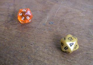
The last of 200 rolls. Could they have been any more bland?
Once you come up with one set of results, you’ll want to verify them. The scientific method, after all, is all about predictability. If this die is biased, it will continue to be biased outside of the game. I’ll roll 200 times—ten times per side—to see if this result remains. At the same time, I’ll roll another die from my grab-bag, so as to compare the two. I picked out an orange clear die. For all 200 of these rolls, I’ve literally rolled both the honey die and the orange die at the same time for 200 throws. The things I will do for this blog!
Let’s look at the orange die first:
- orange = c(4, 5, 19, 4, 6, 16, 20, 4, 6, 5, 13, 3, 1, 13, 2, 17, 9, 14, 10, 8, 18, 10, 4, 9, 9, 4, 20, 7, 16, 13, 12, 4, 17, 6, 11, 3, 19, 9, 19, 2, 6, 19, 18, 17, 20, 9, 4, 6, 6, 16, 5, 4, 14, 13, 8, 16, 18, 17, 5, 18, 9, 11, 14, 8, 18, 8, 16, 8, 6, 20, 20, 9, 20, 3, 1, 13, 8, 10, 2, 4, 2, 15, 3, 4, 14, 7, 6, 16, 18, 7, 5, 1, 10, 5, 4, 19, 18, 9, 6, 7, 2, 3, 15, 4, 3, 3, 10, 12, 6, 7, 1, 5, 20, 8, 8, 2, 7, 15, 2, 8, 18, 16, 7, 6, 19, 14, 10, 4, 9, 1, 17, 13, 6, 17, 4, 7, 7, 20, 8, 4, 20, 19, 17, 13, 7, 17, 18, 3, 1, 9, 4, 7, 9, 16, 6, 3, 1, 14, 10, 2, 8, 10, 14, 5, 3, 11, 12, 16, 19, 4, 7, 18, 16, 6, 6, 12, 19, 15, 13, 16, 18, 11, 14, 17, 19, 6, 16, 18, 18, 10, 6, 11, 18, 10, 20, 12, 15, 2, 2, 9)
- orangefrequency = table(orange)
- orangefrequency
| 1 | 2 | 3 | 4 | 5 | 6 | 7 | 8 | 9 | 10 | 11 | 12 | 13 | 14 | 15 | 16 | 17 | 18 | 19 | 20 |
| 7 | 10 | 10 | 17 | 8 | 17 | 12 | 11 | 12 | 10 | 5 | 5 | 8 | 8 | 5 | 12 | 9 | 14 | 10 | 10 |
That certainly looks pretty random, and the chi-square test agrees.
[toggle code]
- probability = rep(1/20, 20)
- chisq.test(orangefrequency, p=probability)
- Chi-squared test for given probabilities
-
data: orangefrequency<br />
- X-squared = 22.4, df = 19, p-value = 0.2648
Over a quarter of the time we would expect to get results more extreme than these.
Now, what about the honey d20?
- honey = c(8, 19, 15, 6, 3, 15, 4, 1, 14, 17, 16, 8, 3, 15, 15, 3, 10, 5, 1, 8, 13, 8, 1, 16, 13, 20, 4, 1, 11, 10, 6, 18, 10, 1, 6, 4, 11, 2, 19, 9, 18, 13, 20, 19, 6, 13, 20, 4, 5, 19, 3, 5, 15, 1, 18, 20, 7, 8, 16, 11, 4, 18, 7, 9, 17, 15, 7, 5, 19, 11, 18, 7, 18, 4, 18, 18, 12, 12, 2, 9, 1, 5, 15, 15, 10, 17, 3, 2, 14, 3, 1, 13, 7, 5, 1, 12, 8, 16, 8, 10, 11, 18, 9, 16, 6, 11, 4, 11, 16, 10, 5, 9, 10, 10, 10, 17, 15, 10, 1, 19, 20, 13, 16, 13, 11, 5, 9, 4, 7, 19, 7, 13, 7, 14, 20, 19, 17, 3, 2, 10, 13, 10, 19, 18, 8, 11, 12, 7, 2, 11, 5, 8, 11, 5, 1, 20, 9, 10, 9, 11, 20, 15, 14, 4, 2, 15, 17, 13, 5, 4, 1, 7, 5, 9, 7, 17, 15, 19, 20, 19, 15, 20, 1, 4, 1, 5, 9, 18, 18, 9, 13, 1, 4, 20, 2, 1, 18, 3, 16, 10)
- honeyfrequency = table(honey)
- honeyfrequency
| 1 | 2 | 3 | 4 | 5 | 6 | 7 | 8 | 9 | 10 | 11 | 12 | 13 | 14 | 15 | 16 | 17 | 18 | 19 | 20 |
| 16 | 7 | 8 | 12 | 13 | 5 | 11 | 9 | 11 | 14 | 12 | 4 | 11 | 4 | 13 | 8 | 7 | 13 | 11 | 11 |
[toggle code]
- probability = rep(1/20, 20)
- chisq.test(honeyfrequency, p=probability)
- Chi-squared test for given probabilities
-
data: honeyfrequency<br />
- X-squared = 21.6, df = 19, p-value = 0.3046
Even with that run of ones towards the end that resulted in there being yet again more ones than any other result, this is a perfectly reasonable set of rolls: 30% of the time we would expect more extreme results than in this test set of 200. That’s a far cry from the previous results for this die. What does this mean?
Perhaps this confirms the hypothesis that dice rolled in the game are different than dice rolled out of the game. Or, perhaps I’m psychic—I know you’re thinking that. Or it could be that I just happened upon a biased-looking set of rolls while writing this article. It would be just my luck.
Because the first results are not obviously repeatable, I should run some more tests. My arm is tired, however, so I’m not going to. I may do it later on—or ask someone else to do it—after I send the Adventure Guide these results.
Charting the results
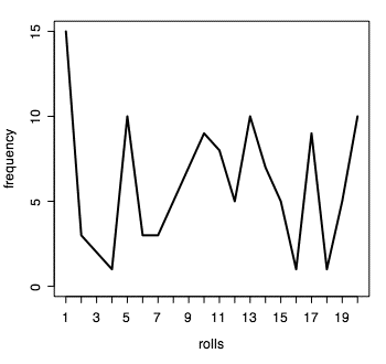
You can also create line charts of your results.
Above, we showed the frequencies of each roll with table(rolls), or in our case just “frequency” since we did frequency=table(rolls). But we can also plot the results on a chart.
The simplest plot is created using:
- plot(frequency)
This will create a chart very much like the lead-in histogram in this article. The full line for creating that chart is:
- plot(frequency, type="h", col="light green", lwd=5, col.axis="red", col.lab="dark green", xlab="d20 rolls")
This gives us a light green color for the data, 5-pixel line widths, a red axis on the left, dark green labels, and a bottom label of “d20 rolls”.
In this latter case I specify a type of “h”, or histogram. That generally makes the most sense for charting dice results. But you might also use:
- plot(frequency, type="l")
This changes to a line chart. Other types include “p” for points, “b” or “o” for both lines and points, and “s” or “S” for stairs.
Statistics
You can also get the minimum and maximum frequency with range(frequency) or the minimum and maximum roll with range(rolls). And sum(frequency) will give you the total number of rolls, because each entry in frequency is the number of times a result came up. Add them together, and that’s the total number of rolls.
You can get the average using mean(frequency) or mean(rolls). If you want the median, you can use median(frequency) or median(rolls). The median is the “middle” number, if you lay out all of the numbers in a row from lowest to highest. If you’re familiar with quantiles, you can use quantile(frequency) or quantile(rolls).
In each case, running it on “frequency” gets you the stats for the number of times numbers come up, and running it on “rolls” gets you the stats for the numbers that were rolled. For example, on the data above, median(rolls) tells me that the median roll was 11; that (or 10) is what we would expect. The mean for the above rolls is 10.47; that’s very close to the 10.5 we’re expecting. If the in-game rolls are biased, it doesn’t appear to be affecting the median or average.
Arbitrary categories
You can use cut to divide the rolls (or frequencies) into arbitrary categories. For example, if you want to count up the number of good rolls and bad rolls, you first have to decide what makes a good roll and a bad roll. Let’s say that rolling five or less is a good roll, and rolling 16 or more is a bad roll.
- cutoffs = c(0, 5, 15, 20)
- qualities = c("Good", "Boring", "Bad")
- rollquality = cut(rolls, cutoffs, qualities)
- table(rollquality)
| Good | Boring | Bad |
|---|---|---|
| 31 | 62 | 26 |
The cutoffs are basically a range. There will always be one more cutoff number than cutoff name. Here, we’re saying that the first category is for numbers greater than zero and up to five. The second category is for numbers greater than five and up to 15. The third category is for numbers greater than 15 and up to 20.
This gives a result of 31 good rolls (1, 2, 3, 4, and 5) and 26 bad rolls (16, 17, 18, 19, 20). There are 62 rolls in between, which we’re calling “boring” rolls.
If you wanted to categorize the rolls more precisely, you might use:
- cutoffs = c(0, 3, 7, 13, 17, 20)
- qualities = c("Great", "Good", "Boring", "Bad", "Awful")
- rollquality = cut(rolls, cutoffs, qualities)
- table(rollquality)
| Great | Good | Boring | Bad | Awful |
|---|---|---|---|---|
| 20 | 17 | 44 | 22 | 16 |
If you want to verify those categories, or if you want to see the rolls in order for some other reason, you can type:
- sort(rolls)
| 1 | 1 | 1 | 1 | 1 | 1 | 1 | 1 | 1 | 1 | 1 | 1 | 1 | 1 | 1 | 1 | 2 | 2 | 2 |
|---|---|---|---|---|---|---|---|---|---|---|---|---|---|---|---|---|---|---|
| 19 | 3 | 3 | 4 | 5 | 5 | 5 | 5 | 5 | 5 | 5 | 5 | 5 | 5 | 6 | 6 | 6 | 7 | 7 |
| 37 | 7 | 8 | 8 | 8 | 8 | 8 | 9 | 9 | 9 | 9 | 9 | 9 | 9 | 10 | 10 | 10 | 10 | 10 |
| 55 | 10 | 10 | 10 | 10 | 11 | 11 | 11 | 11 | 11 | 11 | 11 | 11 | 12 | 12 | 12 | 12 | 12 | 13 |
| 73 | 13 | 13 | 13 | 13 | 13 | 13 | 13 | 13 | 13 | 14 | 14 | 14 | 14 | 14 | 14 | 14 | 15 | 15 |
| 91 | 15 | 15 | 15 | 16 | 17 | 17 | 17 | 17 | 17 | 17 | 17 | 17 | 17 | 18 | 19 | 19 | 19 | 19 |
| 109 | 19 | 20 | 20 | 20 | 20 | 20 | 20 | 20 | 20 | 20 | 20 |
You can see 16 rolls that are 18, 19, or 20 (awful rolls) and 20 rolls that are 1, 2, or 3 (great rolls).
You can use sort on tables as well:
- sort(frequency)
| 4 | 16 | 18 | 3 | 2 | 6 | 7 | 8 | 12 | 15 | 19 | 9 | 14 | 11 | 10 | 17 | 5 | 13 | 20 | 1 |
| 1 | 1 | 1 | 2 | 3 | 3 | 3 | 5 | 5 | 5 | 5 | 7 | 7 | 8 | 9 | 9 | 10 | 10 | 10 | 15 |
This shows which rolls were rolled least often and which were rolled most often.
Examining computer-generated rolls
We can have R generate some random rolls for us.
- rolls = sample(20, 200, replace=TRUE)
- frequency = table(rolls)
| 1 | 2 | 3 | 4 | 5 | 6 | 7 | 8 | 9 | 10 | 11 | 12 | 13 | 14 | 15 | 16 | 17 | 18 | 19 | 20 |
| 6 | 8 | 12 | 9 | 13 | 12 | 8 | 7 | 12 | 11 | 13 | 11 | 8 | 10 | 9 | 10 | 8 | 10 | 7 | 16 |
First, generate 200 rolls from 1 to 20. We have to specify replace=TRUE because by default results taken from a sample are not replaced. That is, it is assuming something like a deck of cards rather than a die. When you pull a card from a deck of cards, you won’t see that card again on subsequent pulls. With dice, however, you will see that number again on subsequent rolls.
When you look at the frequency, make sure that each number from 1 to 20 shows up at least once. In the list above, each number shows up at least once so I’m good to go. Since your list will be different from mine, you’ll need to double-check that all 20 entries show up before going to the next step.
- probabilities = rep(1/20, 20)
- chisq.test(frequency, p=probabilities)
My p-value is 0.8856, making this computer-generated die a non-biased d20.
Always remember that the chi-square test is all about distribution. If the results are somehow related, the chi-square test is simply invalid: it requires that the results--in our case, the die rolls--are unrelated.
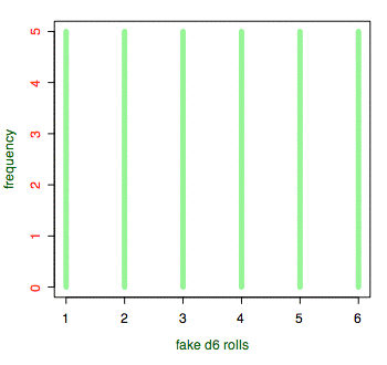
These d6 were created completely non-randomly, ensuring that each number appears exactly the same number of times.
An example of a completely non-random set of results with “random” distribution would be if our computer die roller remembered the last roll, and always switched up to the next option, wrapping around to the bottom once it reaches the highest result. This hypothetical computer-generated d6 would give us 1, 2, 3, 4, 5, 6, 1, 2, 3, 4, 5, 6, etc. Roll it 30 times and you will get each number five times. We can do this in R:
- rolls = c(rep(c(1:6), 5))
- frequency = table(rolls)
- plot(frequency)
- probabilities = rep(1/6, 6)
- chisq.test(frequency, p=probabilities)
Giving us a p-value of 1.0! Which is obviously true: 100% of the time, a truly random die will produce a result more extreme than this. We know these results are non-random, because we know that each “roll” is related to the previous one. If a computer program is doing something behind the scenes to ensure an even distribution of numbers, the chi-square test will not necessarily show us this. Fortunately, this kind of behind-the-scenes manipulation is not something we have to worry about with physical dice, unless Einstein was wrong and God is teasing us.
Plotting a 3d6 roll
As long as we’re playing around, we can look at the “normal distribution” that shows up in early gaming manuals, usually when discussing 3d6 rolls.
I’m far from an expert in R, having learned it specifically for this article, but the easiest way that I could find to generate 3d6 rolls in R is to generate three lists of d6 rolls and add them together.
- samplesize = 50
- roll1 = sample(6, samplesize, replace=TRUE)
- roll2 = sample(6, samplesize, replace=TRUE)
- roll3 = sample(6, samplesize, replace=TRUE)
- rolls = roll1+roll2+roll3
- frequency = table(rolls)
- plot(frequency, type="l", xlab="3d6 rolls")
Change the samplesize from 50 to 500, 5000, 50000, and even 500000, and watch as the line chart smooths out into the “normal distribution” or “bell curve”. As you can see, the difference between 500 rolls and 500,000 is obvious. The more rolls you make, the closer you get to the normal distribution curve. You may want to have a grad student do the actual 500,000 rolls, however.
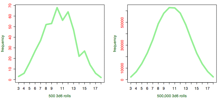
With a carpal tunnel-inducing 500,000 rolls, the distribution looks like the standard normal distribution curve.
- June 27, 2018: Command-line Die Square
-
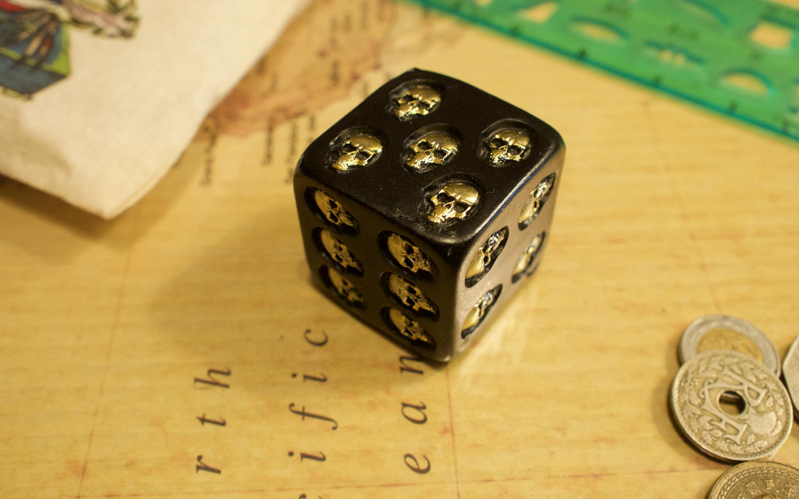
Is it any surprise that a die covered in skulls is biased?
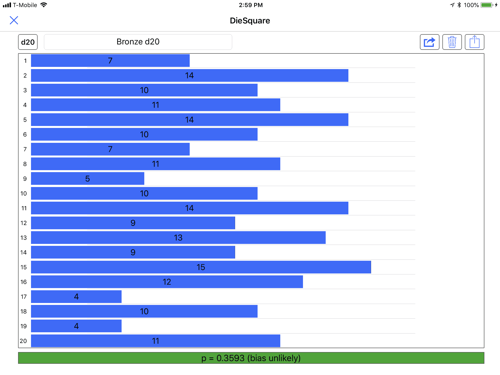
Because Pythonista does not contain scipy, calculating chi-square values using it can have trouble on edge cases. This command-line script can run on data files created by the DieSquare mobile app, and uses scipy to make more reliable calculations.
Specify the DieSquare data file on the command line.
- $ ~/bin/diesquare "Bronze d20.diesquare"
- Degrees of freedom: 19.0 X-square: 20.6
- p-value: 0.359317617197
- d20 bias is unlikely.
You can also specify the die size and a file of tab-delimited or colon-delimited data. The file should contain two columns: the result, and how many of those results occurred.
The DieSquare file format is:
- d6
- 1: 3
- 2: 16
- 3: 9
- 4: 8
- 5: 6
- 6: 18
That is, any line beginning with a lower-case “d” is assumed to be specifying the die size; any line with a number followed by a colon and space followed by a number is assumed to be a result. You can also put comments in by preceding the line with a pound symbol (#).
And as you might guess, this die is almost certainly biased.
- $ ~/bin/diesquare "Skull d6.diesquare"
- Degrees of freedom: 5.0 X-square: 17.0
- p-value: 0.00449979697797
- d6 bias is probable.
The code itself (Zip file, 1.6 KB) is very simple.
[toggle code]
- #!/usr/bin/python
- #http://godsmonsters.com/Features/my-dice-random/diesquare-ios/command-line-die-square/
- import argparse
- import scipy.stats
- parser = argparse.ArgumentParser(description='Calculate Chi Square p-value using DieSquare data files.')
- parser.add_argument('--die', type=int, help='die size')
- parser.add_argument('data', type=argparse.FileType('r'), nargs=1)
- parser.add_argument('--verbose', action='store_true')
- args = parser.parse_args()
-
class ChiSquare():
-
def __init__(self, die, rolls):
- self.die = die
- self.parseRolls(rolls)
-
def parseRolls(self, rolls):
- self.rollCount = 0
- self.rolls = {}
-
for roll in rolls:
-
if not roll:
- continue
-
if roll.startswith('d'):
- self.die = int(roll[1:])
- continue
-
if roll.startswith('#'):
- continue
-
if not roll:
-
if args.verbose:
- print(self.rollCount)
- print(self.rolls)
-
def calculate(self):
-
if args.verbose:
- print '\n# ', self.die
- expected = float(self.rollCount)/float(self.die)
- freedom = float(self.die - 1)
- observed = self.rolls.values()
- expected = [expected]*self.die
- chisquare, pvalue = scipy.stats.chisquare(observed, expected)
- print "Degrees of freedom:", freedom, "X-square:", chisquare
- print "p-value:", pvalue
-
if args.verbose:
-
def __init__(self, die, rolls):
- calculator = ChiSquare(args.die, args.data[0])
- calculator.calculate()
Half of the code is just parsing the datafile; the actual calculation is a couple of lines using scipy:
- observed = self.rolls.values()
- expected = [expected]*self.die
- chisquare, pvalue = scipy.stats.chisquare(observed, expected)
The variable “observed” is the list of observed result counts. The variable “expected” is the list of expected result counts. For example, rolling a d6 60 times, the expected result count is 10 for each result, so expected will equal “[10, 10, 10, 10, 10, 10]”. And observed will be the actual results; for example, in the above data the die face 1 was rolled three times, 2 sixteen times, 3 nine times, 4 eight times, 5 six times, and 6 eighteen times. This is the list “[3, 16, 9, 8, 6, 18]”. The script, of course, uses the lists it constructed by reading the datafile.
- May 16, 2018: DieSquare for iOS
-
Ole Zorn’s Pythonista for iOS is an amazing mobile development environment. If you can do it in base Python, you can do it, inside a GUI, on your iPhone or iPad. This makes it a great tool for gamers who are also programmers.
My dice always seem to be conspiring against me, which is a big reason I’m interested in running chi-square tests. R is an amazing tool for doing so, but it isn’t an amazing tool for entering the data. Last week, after yet another accusation from my teammates that my die is clearly biased to roll low—in a D&D 5 game, where high is better—I started to think they might be right. The first time the accusation was made, I said, look, it’s just because the die knows I’m attacking. I’m going to roll it right now for no reason whatsoever, and the die will come up 20. It did. The die isn’t biased to roll low, it’s biased against me. But it just kept failing.
I thought I’d better double check. Because I am a typical superstitious gamer, I have different dice for different purposes, and this is in fact the first time I’ve used this die—I had it reserved for playing rather than gamemastering. It occurred to me that, since I wrote Are my dice random? in 2006, I have acquired both a great mobile device and a great development environment for it. Wouldn’t it be nice to be able to bring up a table of possible rolls, and tap on each possibility when it came up on the die so as to keep track of each count? That would make rolling through a chi-square test dead easy.
- The R Project for Statistical Computing
- “R is a language and environment for statistical computing and graphics. R provides a wide variety of statistical and graphical techniques, and is highly extensible.”
- When Dice Go Bad
- Martin Ralya isn’t superstitious about dice. That’s why he buried this particular set after a series of bad rolls.
More Best of Biblyon
- Secular Humanist Pantheon
- The Secular Humanist cult, while often oppressed, attracts intelligent, creative worshippers who subscribe to a rich and storied mythology. It will make a great addition to your role-playing game alongside more commonly-role-played mythologies such as Christianity, Buddhism, and Bokonism.
- Why do we need open source games?
- If game rules cannot be copyrighted, and if compatible supplements require no permission, what is the point of an open content game book? Over the next three installments, I’ll look at how open content licenses can make for better gaming.
- Experience and Advancement in Role-Playing Games
- Kill monsters. Take their stuff. How has character advancement in role-playing games changed over the years? Starting with original D&D and on up through a handful of modern games, I’ll be surveying methods of experience and character advancement over the years.
- Spotlight on: Evil
- No one considers themselves Evil. So how does the Evil moral code relate to the game of Gods & Monsters? How and why do Evil non-player characters act?
- Populating England
- Use the history of England as an example of how to steal ideas from real history for your game world.
More chi-square
- Command-line Die Square
- Running chi-square on the command-line, using data from the mobile Pythonista app.
- DieSquare for iOS
- Are your dice biased? Perform on-the-fly chi-square tests using your iPad or iPhone and Pythonista.
More gaming tools
- First level calculations in Pocket Gods
- If you need to quickly calculate reactions and other numbers for a first level character, Pocket Gods can now do that for you.
- Roll20 and Gods & Monsters
- Roll20 appears to easily accept the Inkscape maps I’ve been creating for the various Gods & Monsters adventures
- Automatically grab flavor text snippets in Nisus
- In Nisus, it is very easy to grab all text of a specific style, and its nearest heading. This makes it easy to make “room description cards” for handing to the players after reading them.
- hexGIMP for old-school wilderness maps
- The isoMage has a script and brushes for GIMP that make it easy to create old-school TSR-style outdoor maps.
- Constructing encounter tables using Nisus
- Here’s a Nisus Writer macro that makes it a little easier to create encounter tables.
- 13 more pages with the topic gaming tools, and other related pages
More Programming for Gamers
- Programming for Gamers: Choosing a random item
- If you can understand a roleplaying game’s rules, you can understand programming. Programming is a lot easier.
- Easier random tables
- Rather than having to type --table and --count, why not just type the table name and an optional count number?
- Programming a Roman thumb
- Before we move on to more complex stuff with the “random” script, how about something even simpler? Choose or die, Bezonian!
- Multiple tables on the same command
- The way the “random” script currently stands, it does one table at a time. Often, however, you have more than one table you know you’re going to need. Why not use one command to rule them all?
- How random is Python’s random?
- Can you trust a script’s random number generator to actually be random?
- 12 more pages with the topic Programming for Gamers, and other related pages
More randomness
- While sorrowful dogs brood: The TRS-80 Model 100 Poet
- Random poetry: a BASIC random primer and a READ/DATA/STRINGS primer, for the TRS-80 Model 100.
- How random is Python’s random?
- Can you trust a script’s random number generator to actually be random?
